How To Draw Phase Portraits Of Nonlinear Systems

Phase Portraits of Nonlinear Systems

Consider a $2 \times 2$ , perhaps nonlinear, autonomous system $x' = f(x,y)$ , $y' = g(x,y)$ (autonomous means that the independent variable $t$ , thought of as representing time, does not occur on the right sides of the equations). Merely every bit we did for linear systems, nosotros want to look at the trajectories of the system. Since in most cases information technology is impossible to solve these systems exactly, we will concentrate on the qualitative aspects, and in particular on how to sketch the phase portrait by manus.

Here are some of the principles of trajectory sketching:

The linear approximation to a part of 2 variables $f(x,y)$ about a indicate $(a,b)$ is

$\begin{displaymath}f(x,y) \approx f(a,b) + (x-a) \frac{\partial f}{\partial x}(a,b) + (y-a) \frac{\partial f}{\partial y}(a,b) \end{displaymath}$

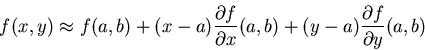
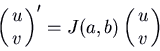
Nosotros desire to practise this in item at an equilibrium point, where $f(a,b) = g(a,b) = 0$ . It is useful to make a change of variables $u = x-a$ , $v = y-b$ , so $u=0$ , $v=0$ corresponds to the equilibrium point. Then the linearization of our organisation at this equilibrium signal is the $2 \times 2$ constant-coefficient linear homogeneous system

$\begin{displaymath}\pmatrix{u\cr v\cr}' = J(a,b) \pmatrix{u\cr v\cr} \end{displaymath}$

where the matrix

$\begin{displaymath}J = \pmatrix{ \partial f/\partial x & \partial f/\partial y\cr \partial g/\partial x & \partial g/\partial y\cr}\end{displaymath}$

is called the Jacobian of the vector field $(f,g)$ .

Example: Consider the system

$x' = x (y - 1)$ ,

$y' = y (x-1)$ .

For an equilibrium point we need $x (y-1) = 0$ (i.e. $x=0$ or $y=1$ ) and $y (x-1) = 0$ (i.east. $y=0$ or $x=1$ ). At that place are thus ii equilibrium points: $(0,0)$ and $(1,1)$ .

Before classifying the equilibrium points, it's a good thought to describe the isoclines for $x' = 0$ and $y'=0$ . I'll plot the get-go in bluish and the second in green. I indicate with arrows the direction field in each region and on the isoclines. The intersections of the blueish and dark-green isoclines are the equilibrium points.

The Jacobian matrix is 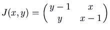$\displaystyle J(x,y) = \pmatrix{ y-1 & x\cr y & x-1 \cr}$ . At the equilibrium point $(0,0)$ this is $\displaystyle \pmatrix{ -1 & 0\cr 0 & -1\cr}$ . That has a double eigenvalue $-1$ , and two linearly contained eigenvectors. Therefore the equilibrium point $(0,0)$ is a atypical node, and is an attractor.

At the 2d equilibrium point $(1,1)$ the Jacobian matrix is $\displaystyle \pmatrix{0 & 1\cr 1 & 0\cr}$ . This has eigenvalues i and $-1$ . Therefore the equilibrium bespeak $(1,1)$ is a saddle. The eigenvectors are $\displaystyle \pmatrix{1\cr 1\cr}$ for 1 and $\displaystyle \pmatrix{-1\cr 1\cr}$ for $-1$ . The picture beneath shows the phase aeroplane with some parts of trajectories near the two equilibrium points. Note that the directions of these trajectories agree with the management field arrows from the previous movie.

Now nosotros sketch some trajectories. There are trajectories on the $x$ and $y$ axes (going in to the equilibrium point at the origin), because $x' = 0$ when $x=0$ and $y'=0$ when $y=0$ . Next it'due south a good idea to sketch the trajectories coming out of and going in to the saddle point. For instance, 1 comes in to the saddle point from beneath and to the right. We go backwards in time, following the arrows backward. These arrows point up and left in the region $x > 1$ , $0 < y < 1$ . The trajectory must curve to avert the trajectory on the positive $x$ centrality. It is presumably asymptotic to that axis. The trajectory coming out of the saddle bespeak downward and to the left must proceed down and to the left until it ends at the equilibrium betoken $(0,0)$ .

Finally, we draw some more trajectories, including at least one in each region. Annotation that those trajectories that enter the equilibrium point at $(0,0)$ can practice and then at any angle.

Our picture is symmetric about the line $x=y$ , because of the fact that the arrangement of equations remains the same if you interchange $x$ and $y$ .

The trajectories entering and leaving the saddle point are separatrices. All trajectories below and to the left of the two trajectories entering the saddle go to the equilibrium point $(0,0)$ equally $t \to \infty$ , while those above and to the right become off to infinity asymptotic to the line $x=y$ . Below and to the right of the trajectories leaving the saddle, everything comes in from infinity asymptotic to the positive $x$ centrality (as $t \to -\infty$ ), while in a higher place and to the left of these everything comes in from infinity asymptotic to the positive $y$ axis.

As I mentioned, in that location are two exceptions to the rule that the phase portrait about an equilibrium indicate can be classified by the linearization at that equilibrium point. The offset is where 0 is an eigenvalue of the linearization (nosotros didn't even look at the linear organisation in that example!). The second exception is where the linearization is a center. The linear organization has periodic solutions, respective to trajectories that are closed curves (ellipses). Imagine starting at some point and following the direction field. Afterward going all the mode around the equilibrium betoken, in the linear organization you return exactly to the point yous started at. This is a very delicate matter, and any nonlinear effect, fifty-fifty if very pocket-size, could spoil it. If in the nonlinear organization you come up back slightly farther away from the equilibrium point than where you started, and then your trajectory can non exist a airtight bend. The adjacent time around, you will be still farther away. The trajectory will spiral away from the equilibrium bespeak. If all trajectories about the equilibrium point are like this, the equilibrium point is an unstable screw. On the other paw, if later on one plow around the equilibrium point you are slightly closer than where y'all started, your trajectory spirals inwards. If all trajectories near the equilibrium betoken are like this, the equilibrium point is a stable spiral (and an attractor). Here are pictures of those two possibilities. The 3rd possibility, of course, is that you do come dorsum exactly to the point where you started, and it really is a centre.

One fashion to show that a center of the linearized arrangement is nonetheless a centre in the nonlinear system is to find an equation for the trajectories. If in that location is such an (implicit) equation $F(x,y) = c$ where $F$ is a smoothen function, not constant in whatsoever region, and $c$ an arbitrary constant, then the trajectories, which are level curves of this function, tin non be spirals simply tin can be closed curves. This occurs both in the predator-prey and pendulum systems.